Basic Performance Models for Matrix-Matrix Product.
Performance modeling is the way we can measure how good is our application. There are two essentials ways to measure our application:
- An analytic expression based on the application code.
- An analytic expression based on the application’s algorithm and data structures.
The reason is that we are looking to extrapolate our application to a large scale computers, too see how scalable the application is. Also, we want to identify possible inefficiencies in compilation/runtime or mismatch in developer expectations.
Matrix-Matrix Multiplication Example:
Let A and B be nxn matrixes.
\[A= \begin{bmatrix} a_{11}& a_{12} & \ldots &a_{1n}\\ a_{21}& a_{22} & \ldots & a_{2n}\\ \vdots& \ldots & \ddots & \vdots\\ a_{n1}& a_{n2} & \ldots &a_{nn} \end{bmatrix} \space \space B= \begin{bmatrix} b_{11}& b_{12} & \ldots &b_{1n}\\ b_{21}& b_{22} & \ldots & b_{2n}\\ \vdots& \ldots & \ddots & \vdots\\ b_{n1}& b_{n2} & \ldots &b_{nn} \end{bmatrix}\]If we want to perform the product between them, classically we would:
-
Take one-by-one the lines from matrix A. For example, for the first line:
\[\begin{bmatrix} a_{11}& a_{12} & \ldots &a_{1n} \end{bmatrix}\] -
Take one-by-one the Columns from matrix B. In the case of the first line:
\[\begin{bmatrix} b_{11}\\ b_{21}\\ b_{31}\\ \vdots\\ b_{n1}\\ \end{bmatrix}\] -
Perform the operation and assign the result to the position \(c_{11}\) in the matrix result \(C_{nxn}\):
Repeat for every line and column. In fortran-like:
#Pseudocode for Fortran:
    do i=1, n
        do j=1,n
            c(i,j) = 0
            do k=1,n
             c(i,j) = c(i,j) + a(i,k) * b(k,j)
In order for us to calculate how much computing time this task takes, we need to calculate the number of basical steps that it takes i.e we will count each operation as a indicator of the number of steps.
Following the example, we have:
- For the multiplication in each possition we have:
- n multiplications
- n-1 sums
- In total we can say we have \(n+(n-1)\sim 2n\) operations
- We have \(n^2\) elements in the matrix.
In conclusion it takes \(2(n^3)\) Operations to multiply matrixes using the clasical ways. There are different algorithms that have proved to be faster. In fact the faster algorithm takes \(O(n^{2.373})\) Williams, 2014.
Now. I have a MacBook Air with a 1.4 Ghz processor. ( These are the configurations). That means The number of floating point operations are given by:
1
FlOP/S : Floating Point Operations Per Second
So that, to perform a n=100 matrix multiplication would take:
\(2(100)^3= 2 \times 10^6 operations\) and
\(Time= \frac{2 \times 10^6}{1,4 \times 10^9}= 1.4 \times 10^{-3} seconds\).
For n=1000 we should expect then:
\[2(1000)^3 = 2 \times 10^9 operations\] \[Time= \frac{2 \times 10^9}{1,4 \times 10^9}= 1.4 sec\]So on and so far.
Upss!
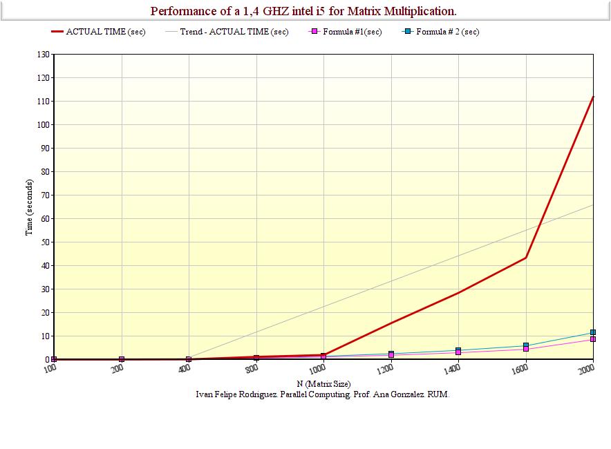
I just wanted to be sure, so I ran the code. This was the actual performance I obtained.
Let be \(2n^3\) the order for matrix multiplication. One can assume the total time can be expressed by:
\[Time = 2kn^3\]Therefore,
\[k= \frac{Time}{2n^3}\]Were k is a constant.
The formulas used for prediction were:
-
Formula #1: This formula was obtained taking the first value (N=100) to find a k. And then using the formula explained before.
\[k=\frac{1,06\times 10^{-03} }{2\times 10^{+06}}=5,3\times 10^{-10}\] -
Formula #2: This formula was taken by the theoretically clockspeed of my machine. Knowing that it is a 1,4GHz processor, I got:
\[K = \frac{1}{1,4\times 10^{+09}}=7,14\times 10^{-10}\]
| N | Measured Performance MFLOP/s | Measured Time (sec) | Formula Time #1 | Formula Time #2 |
|---|---|---|---|---|
| 100 | 1,89E+03 | 1,06E-03 | 1,06E-03 | 1,4E-03 |
| 200 | 1,89E+03 | 8,46E-03 | 8,48E-03 | 1,1E-02 |
| 400 | 1,72E+03 | 7,46E-02 | 6,78E-02 | 9,1E-02 |
| 800 | 9,10E+02 | 1,13E+00 | 5,43E-01 | 7,3E-01 |
| 1000 | 1,04E+03 | 1,92E+00 | 1,06E+00 | 1,4E+00 |
| 1200 | 2,23E+02 | 1,55E+01 | 1,83E+00 | 2,5E+00 |
| 1400 | 1,93E+02 | 2,84E+01 | 2,91E+00 | 3,9E+00 |
| 1600 | 1,89E+02 | 4,33E+01 | 4,34E+00 | 5,9E+00 |
| 2000 | 1,43E+02 | 1,12E+02 | 8,48E+00 | 1,1E+01 |
Graphically:
If we compare it with the MFLOP/s operation the processor is doing, we see that:
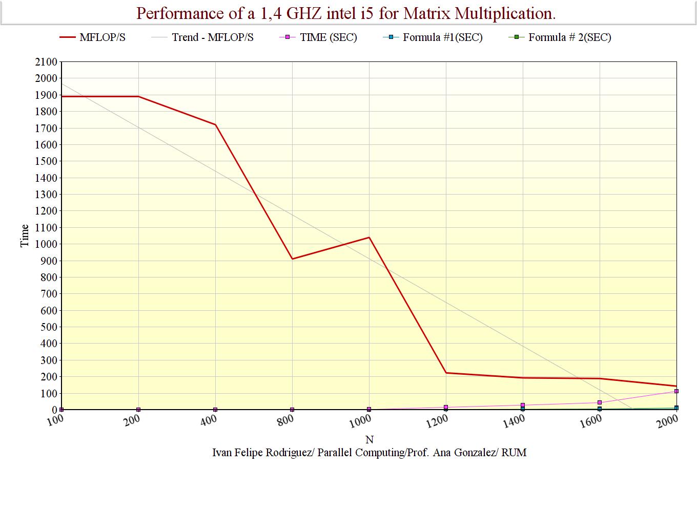
As you can appreciate, the theoretical predictions were not even close but for the cases were N was little. This means there are some characteristics our model is not taking in cosiderantion (Like the latency or bandwith of the memory). For this reason a better model should include variables for the loads and stores the processors needs to make. These tasks made that my processor instead of using the full potency of 1809 MFlop/s only used 143 MFlop/s for the larger N cases.