Hi, I'm Ivan.
I work at the Center for Advanced AI as an Advanced ML/AI Research Manager. My work focuses on agentic AI, RAG, and LLM systems. I hold a PhD in Cognitive Science from Brown University.
Research
Agentic AI · foundation models · multimodal reasoning · neuroscience-inspired learning · robustness & alignment · long-context LLM systems. I also work on aligning deep neural networks with human behavioral decisions and human-like visual representations.
Fossil leaves hold rich data on evolutionary history and ancient ecosystems, but identification remains manual and expert-dependent, leaving most collections as paleobotanical “dark data.” We introduce a deep learning system that generates fossil-like images from modern leaves and aligns family-diagnostic features across modern and fossil specimens. Evaluated on vetted families from Florissant Fossil Beds (Eocene, Colorado), it maintains strong accuracy even when all fossils from a test family are withheld. Concept-based explanations highlight diagnostic morphology—venation, margins, leaf base—to support expert review. On previously unidentified Florissant specimens, the system gives credible family-level hypotheses for 85.6% of specimens.
Explore Leaf Lens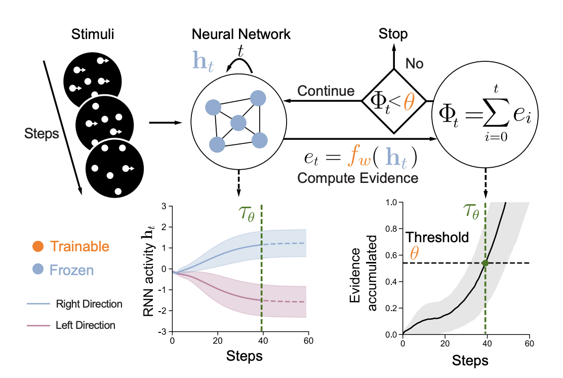
A trainable module that aligns RNN dynamics with human reaction times: a frozen RNN’s hidden state h_t is mapped to evidence e_t = f_w(h_t), accumulated as Φ_t. When Φ_t exceeds a learned threshold θ, processing stops; that time step τ_θ is the model RT. Can be trained with human RT supervision or via self-penalty for speed–accuracy trade-off.
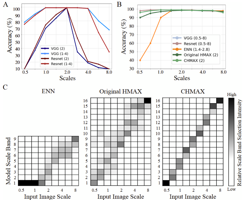
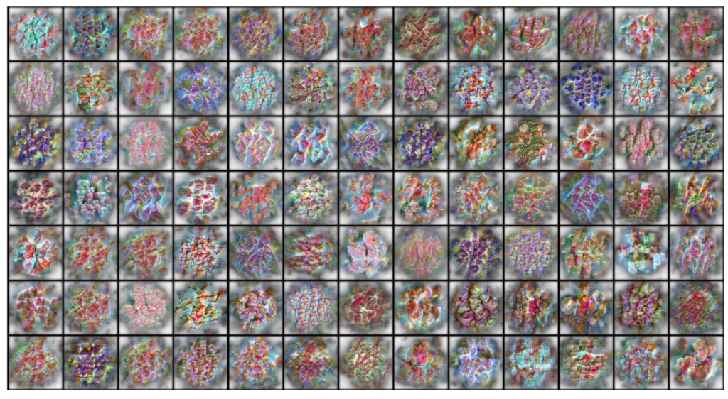
Exploring self-supervised learning approaches to create more human-like visual representations that are scale-invariant and better aligned with biological vision systems.
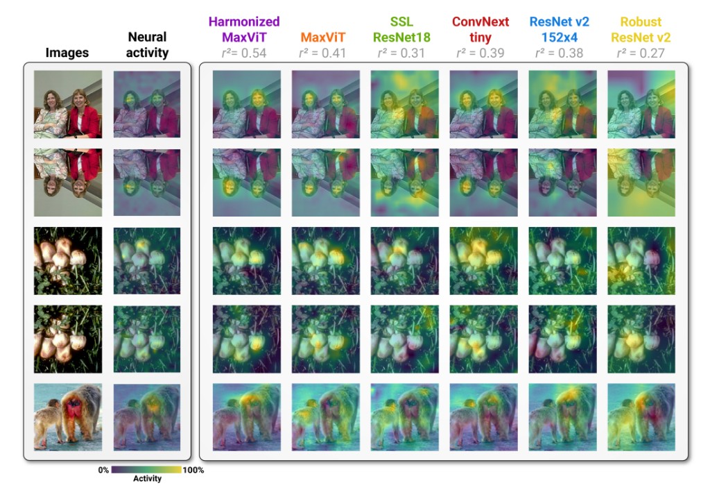
Investigating the trade-off between model performance and biological plausibility, showing that performance optimization can lead to models that are less aligned with human visual processing.
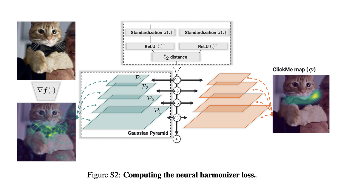
Developing methods to align deep neural networks with human visual strategies, improving both performance and interpretability of computer vision models.
Publications
A selection of my recent publications in computer vision, machine learning, and cognitive science.
Mentoring
I enjoy guiding students in research and helping them achieve their goals. Here are a few of my mentees and what they have accomplished.
Jeffrey studies Data Science at the University of Michigan. He has built projects including Mini-AlphaGo (hybrid AlphaGo/AlphaGo Zero for 9×9 Go with MCTS and bot arena), Tuesday (executive functioning web app for students), and has 4+ years in data science and 5+ years in web development. We collaborated on a conference paper on reading comprehension and logical reasoning.
Ananya has been accepted to Stanford University. She researches cybersecurity for the quantum-computing era and has interned at the Georgia Tech Cyber Forensics Lab. Her work on the impact of NIST's quantum-resistant cryptographic algorithms (CRYSTALS-Kyber, Dilithium, FALCON, SPHINCS+) on website response times—evaluating SSL handshake and download time under varying network conditions—provides empirical evidence to support adoption of quantum-safe cryptography.
arXiv: The Impact of QSC on Website ResponseVaishnav researches AI detection of geospatial deepfakes—AI-manipulated satellite imagery—to improve national satellite security. He trains detection models using GAN-generated data (e.g., SpaceNet 7) and is extending the work with diffusion models. He has presented at the Esri International User Conference (San Diego), met Jack Dangermond (Esri), and was invited to present at the CCIR Student Research Symposium at the University of Cambridge. His work has been featured in outlets such as Danville San Ramon.
Danville San Ramon featureYash was a finalist at the International Science and Engineering Fair (ISEF). His project: “A Novel Comprehensive Tool Utilizing Machine Learning Models for Remote, Cost-Effective, Real-Time Wound Risk Assessment.” Volunteering in a nursing home sparked the idea for building an ML-based tool to assess wound risk in real time for clinical and care settings.