Shared Memory Processors

Parallel computing has been the key tool for high performance computing in the last decade. The idea is to brake a long and hard problem into a several smaller ones that can be executed in different cores, solving the problem in a coperative way[hager][1]. However, being able to guarantee that the portion of cached memory is an accurate copy of main memory is known as cache coherence[Eijkhout][2].

Those computers that use the same physical space address for their processors are known as “shared-memory computers”. In this case there are two very different ways to access memory, with the following caracteristics:

  • Uniform Memory Access (UMA): In this case latency and bandwith is the same for all processors and all memory locations.

  • On cache-coherence Nonuniform Memory Acces (ccNUMA): In this case memory is physically distributed but logically shared. i.e.Each processor would process their own portion of memory, but using a network logic makes it a whole system appears as a one single addres space.

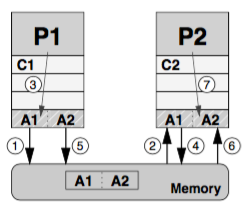
Both of these systems may have multiple CPUs with copies of the same cache line in different caches, probably in modified state. For this reason is necessary to have cache coherence policies that guarantee consistency between cached data and data in memory at all times.

One of the protocols that guarantees the information coherence is the MSI protocol:

  • M modified: The cache line has been modified in this cache, and ir resides in no other cache thant this one. Therefore a cache with a block in “M” state is responsable of writing it back to the memory.
  • S shared: The cache line has been read from a memory but not (yet) modified. There are read-only copies in at least one other cache. The cache can evict data without writing back
  • I invalid: The cache line does not reflect any sensible data. Usually this happens if the cache line was in “S” state but another processor has requested exclusive ownership.
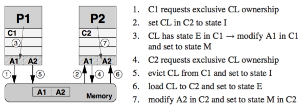
Explanation

Taken from [1]

Resources:

[1] Hager,Wellein. Introduction to High Computing Performance for scientist and engineering. CRC press. pages 27-30 2010

[2] Victor Eijkhout. Introduction to High Performance Scientific Computing. 2011.

[3] https://en.wikipedia.org/wiki/MSI_protocol

*OoO (Out of order)

This example was an exercise proposed by Dr. Rémi Mégret in M6786 Class.

We consider a multi-issued super scalar processor. At each cycle, the following instruction can be issued simultaneosly:

1 load or store + 1 FP addition or substraction + 1 FP multiplication. (FP: Floating Point)

The latencies (pipeline depth) of the instructions are as follows: Load/store : 2 cycles; FP adition: 2 cycles; FP muliplication: 3 cycles.

For simplicity we assume that:

  • All other operations (inicialization,loop/branch, integer arithmetic…) Come at no cost.

  • There is no additional latency with memory (no cache miss)

Therefore only load, FP sub, FP add and FP mult marked in bold in the code will be taken in consideration.

#        i=0
#        R5=0 // Note: R# corresponds to register number # 
   loop: load A[i] into R_1
         sub R_3 = R_2 -R_1
         mult R_4= R_3 * R_3
         add R_5 = R_5 + R_4
#        i=i+1
#        branch to loop if i<N
#        store R5 into s

The chronogram:

There are several ways to represent a pipeline that perform this process. In this case, I will represented it taking in consideration each task (load 1, load 2, sub, mult and add) in a different line, the full instruction will be done after it gets to the bottom of the pipeline. And the next instruction will be read in the columns at the right.

Pipeline Chronogram

No pipeline:

As we observed in the graph. In case that we run a no-pipeline process, we will take 11 cycles to perform just one instruction. Therefore the throughput would be \(\sim\) 0.09 instructions per cycle.

Pipeline.

Now we want to speed up this process and we decide to use a pipeline. The second and third diagram explains this clearly. Though we have to wait eleven cycles (wind-up phase) to have the first output, after that every 3 cycles we will have a new result. Thus, we have improved the troughput almost 300% per cycle. In the same 22 cycles depicted instead of having 2 instructions ready, we have 5.

Note that the pattern starts after the 5th cycle. The reason is that we cannot schedule more substractions in line, because if we do so, after substracting the third element (A[3]-B[3]), we would overwrite its information causing a wrong multiplication at the [4] instruction. That is also why we need to stall the loading unit in the 4th cycle untill that substraction has been processed. Thereafter the pattern is the same.

Troughput.

By definition we will consider troughput as the “amount of work done in a given time” [patterson][1]. In this case we will use the clock cycle of the processor. For instance, the troughput of the first diagram would be: 1/11. Because in a single cycle that portion of the entire instruction is processed. However, in the second diagram we have that every 3 cycles (with n big enough) we have an instruction complete, which represent 0.33 throughput.

In the second and third pipeline the troughput is 3.6 higher than in a no-pipeline processor.

Even though the second and third processor have different scheduling, the throughput does not change. The reason is that the multiplication is the critical operation wich latency, no matter how good I organize the information, is always 3 cycles.

Architecture Diagram.

One possible processor design to perform this operation, would need esentially four components: The Fetch-Decode unit, the load/store, the FP Multiplication and the FP addition/substraction unit. I suggest the following architecture would work efficiently:

Processor architecture

Since we have out-of-order execution is necessary to have a fetch-decode unit that schedule the orders. Then we have a separate unit to perform each of the different task, however only three different operation can take place at each cycle in this processor. In the end there is the commit unit that wraps all the results and reorder them in the right place, to finally store them back in the main memory.

Discussion:

As we appreciated the critical point is related to the multiplication unit. That unit is working all the time, however because of its latency, all the other units are not used to its full potential. Since they have one cycle each of stall.

Performance modeling is the way we can measure how good is our application. There are two essentials ways to measure our application:

  • An analytic expression based on the application code.
  • An analytic expression based on the application’s algorithm and data structures.

The reason is that we are looking to extrapolate our application to a large scale computers, too see how scalable the application is. Also, we want to identify possible inefficiencies in compilation/runtime or mismatch in developer expectations.

Matrix-Matrix Multiplication Example:

Let A and B be nxn matrixes.

\[A= \begin{bmatrix} a_{11}& a_{12} & \ldots &a_{1n}\\ a_{21}& a_{22} & \ldots & a_{2n}\\ \vdots& \ldots & \ddots & \vdots\\ a_{n1}& a_{n2} & \ldots &a_{nn} \end{bmatrix} \space \space B= \begin{bmatrix} b_{11}& b_{12} & \ldots &b_{1n}\\ b_{21}& b_{22} & \ldots & b_{2n}\\ \vdots& \ldots & \ddots & \vdots\\ b_{n1}& b_{n2} & \ldots &b_{nn} \end{bmatrix}\]

If we want to perform the product between them, classically we would:

  1. Take one-by-one the lines from matrix A. For example, for the first line:

    \[\begin{bmatrix} a_{11}& a_{12} & \ldots &a_{1n} \end{bmatrix}\]
  2. Take one-by-one the Columns from matrix B. In the case of the first line:

    \[\begin{bmatrix} b_{11}\\ b_{21}\\ b_{31}\\ \vdots\\ b_{n1}\\ \end{bmatrix}\]
  3. Perform the operation and assign the result to the position \(c_{11}\) in the matrix result \(C_{nxn}\):

\[a_{11}b_{11} + a_{12}b_{21} + \ldots a_{1n}b_{n1}\]

Repeat for every line and column. In fortran-like:

#Pseudocode for Fortran:
    do i=1, n
        do j=1,n
            c(i,j) = 0
            do k=1,n
             c(i,j) = c(i,j) + a(i,k) * b(k,j) 

In order for us to calculate how much computing time this task takes, we need to calculate the number of basical steps that it takes i.e we will count each operation as a indicator of the number of steps.

Following the example, we have:

  • For the multiplication in each possition we have:
    • n multiplications
    • n-1 sums
    • In total we can say we have \(n+(n-1)\sim 2n\) operations
  • We have \(n^2\) elements in the matrix.

In conclusion it takes \(2(n^3)\) Operations to multiply matrixes using the clasical ways. There are different algorithms that have proved to be faster. In fact the faster algorithm takes \(O(n^{2.373})\) Williams, 2014.

Now. I have a MacBook Air with a 1.4 Ghz processor. ( These are the configurations). That means The number of floating point operations are given by:

1
FlOP/S : Floating Point Operations Per Second 
\[1(processor)\times 1,4 \times 10^9 (frecuency)= 1,4 \times 10^9 FLOPS\]

So that, to perform a n=100 matrix multiplication would take:

\(2(100)^3= 2 \times 10^6 operations\) and

\(Time= \frac{2 \times 10^6}{1,4 \times 10^9}= 1.4 \times 10^{-3} seconds\).

For n=1000 we should expect then:

\[2(1000)^3 = 2 \times 10^9 operations\] \[Time= \frac{2 \times 10^9}{1,4 \times 10^9}= 1.4 sec\]

So on and so far.

Upss!

I just wanted to be sure, so I ran the code. This was the actual performance I obtained.

Let be \(2n^3\) the order for matrix multiplication. One can assume the total time can be expressed by:

\[Time = 2kn^3\]

Therefore,

\[k= \frac{Time}{2n^3}\]

Were k is a constant.

The formulas used for prediction were:

  • Formula #1: This formula was obtained taking the first value (N=100) to find a k. And then using the formula explained before.

    \[k=\frac{1,06\times 10^{-03} }{2\times 10^{+06}}=5,3\times 10^{-10}\]
  • Formula #2: This formula was taken by the theoretically clockspeed of my machine. Knowing that it is a 1,4GHz processor, I got:

    \[K = \frac{1}{1,4\times 10^{+09}}=7,14\times 10^{-10}\]
N Measured Performance MFLOP/s Measured Time (sec) Formula Time #1 Formula Time #2
100 1,89E+03 1,06E-03 1,06E-03 1,4E-03
200 1,89E+03 8,46E-03 8,48E-03 1,1E-02
400 1,72E+03 7,46E-02 6,78E-02 9,1E-02
800 9,10E+02 1,13E+00 5,43E-01 7,3E-01
1000 1,04E+03 1,92E+00 1,06E+00 1,4E+00
1200 2,23E+02 1,55E+01 1,83E+00 2,5E+00
1400 1,93E+02 2,84E+01 2,91E+00 3,9E+00
1600 1,89E+02 4,33E+01 4,34E+00 5,9E+00
2000 1,43E+02 1,12E+02 8,48E+00 1,1E+01

Graphically:

Performance of the 1,4 GHz MacBook's Processor

If we compare it with the MFLOP/s operation the processor is doing, we see that:

MFlop/s vs Time

As you can appreciate, the theoretical predictions were not even close but for the cases were N was little. This means there are some characteristics our model is not taking in cosiderantion (Like the latency or bandwith of the memory). For this reason a better model should include variables for the loads and stores the processors needs to make. These tasks made that my processor instead of using the full potency of 1809 MFlop/s only used 143 MFlop/s for the larger N cases.

Out of Order Execution. (Dynamic Execution)

As it was described before, the instructions are stored in the registers and they are loaded from the memory. However, given that nowadays memories are still not quite too fast, is possible that the arguments of such instructions are not available “on time”. For this reason Out of order execution can execute orders that appear later on the instructions but have their parameters ready. This improves instruction throughput and makes it easier for compilers to arrange machine code for optimal performance. [Hager][1].

The basic idea is to keep track of the program order in which instructions entered the pipeline and for each of these instructions, it maintains a temporary register storage.[Balasubramonian][6] This way if is needed later to perform a different operation using some of the instructions or results obtained previously.

Using static (in-order) processors the steps that follows usually are:

  1. Instruction fetch.
  2. If input operands are available (in registers for instance), the instruction is dispatched to the appropriate functional unit. If one or more operands are unavailable during the current clock cycle (generally because they are being fetched from memory), the processor stalls until they are available.
  3. The instruction is executed by the appropriate functional unit.
  4. The functional unit writes the results back to the register file

Using dynamic processors, the steps are:

  1. Instruction fetch.
  2. Instruction dispatch to an instruction queue (also called instruction buffer or reservation stations).
  3. The instruction waits in the queue until its input operands are available.
  4. The instruction is then allowed to leave the queue before earlier, older instructions.
  5. The instruction is issued to the appropriate functional unit and executed by that unit.
  6. The results are queued.
  7. Only after all older instructions have their results written back to the register file, then this result is written back to the register file. This is called the graduation or retire stage. wikipedia

Avoiding the stalls on the processors helps improve considerably the performance. This graph would help us understand why,

Static vs Dynamic scheduling

Taken from: [wright][8]

In larger operations the improvement would impact higher the performance. Cur- rent out-of-order designs can keep hundreds of instructions in flight at any time, using a reorder buffer that stores instructions until they become eligible for execution[1].

Despite the limitations we have discussed in the previous post, in the recent years there has been a great focus on chip design looking to improve some features that let us take the most of them.

Pipelines.

Let us suppose you have a shoes factory. Every shoe takes 2 days in construction if its made by one employee. There are a houndred employees at your factory. You want to have every worker doing his job everytime so you don’t loose money. You decided then, to have every one working on a new shoe by themselves. In this way, every one start today (let’s say monday) and the shoe would be ready by wednesday. Working in this way is inefficient, because you have to wait two days to have shoes ready for distribution. This is the way processors worked before.

Assembly lines

Taken from here: Assembly lines

Now, let us say you call your friend who is a computer scientist. He then counsel you not to have everyone working on their own shoe, but having them in a line working for different part of the shoe. So that one worker would focus only on pasting the shoes, other in cutting the leather, other one to paint, other one to pack, so on and so far. In this way, you will have a consistent production that produces shoes everytime. This is the way processors are working today.

Of course there are some considerations. For example, every worker should finish his job on time, in case that one worker delays the whole production would be delayed too.

Processors manage different instructions for example loads, stores, address calculations, instruction fetch and decode, etc. These instructions can be executed independently,so that they can be distributed on different registers . Like the assembly line, pipelining takes care of having ready data for processing once the operand has finished.

For instance, in the most basic schema “fetch-decode-execute” pipeline, while an instruction is being executed, another one is being decoded and a third one is being fetched from instruction (L1I) cache.[hager][3]. In the assembly line, the first product is the one who takes the most time, because the worker situated at the end of the line must wait untill the production moves up to him, in the processor this is the so called winds-up phase.

Wind-up phase: This is the latency untill the pipeline is ready to execute the orders simuntaneously.

In the case workers need to work on a different shoe, they must need to wait untill the assembly line is empty, to start over, this is the so called winds-down phase.

Winds-down phase: This is the latency untill pipeline executes the last order to have the result ready.

The following image depict this schema more clearly.

Schematic view of a pipeline processing in 2D with 4 processors

Taken from [Deserno et. all][4].

As shown in the previous figure. CPU 1,2,3 need to wait untill the CPU 0 has the calculation ready, to move into CPU 1, now CPU 0 and CPU 1 are working simuntaneously. Once each of them has finished (winds-up), the computation time would turn from 4 cycles to only 1 cycle per operation. In the end, we should wait untill CPU 3 finishes with the last calculation (winds-down). And the full instruction would be fully executed[4].

In general for a pipeline of depth m, executing N independent, subsequent operations takes N+m-1 steps. While in a general purpouse takes mN steps. The versus speed up is given by the formula,

\[\frac{T_{seq}}{T_{pipe}}=\frac{Nm}{N+m-1}\]

Drawbacks and Hazards

Knowing the advantages of subdividing the process in more simpler ones, one might think it would be suitable to add more stages to perform difficult tasks. However there are some risks known as the pipeline hazards basically for the known problem discussed before of the assembling line: It is required that each stage perform its work on time or the whole pipeline would stop. In this way there are at least three different hazards we can think ofkristoffer [5]:

  • Structural Hazards: occur when hardware, such as the memory subsystem, does not support the execution of certain two instructions in parallel.
  • Data Hazards:arise when a needed operand is not ready, because either the current instruction is not finished computing it, or it has not arrived from storage.
  • Control Hazards: occur when it is simply not known which instruction should come next.